Neural Compression Models

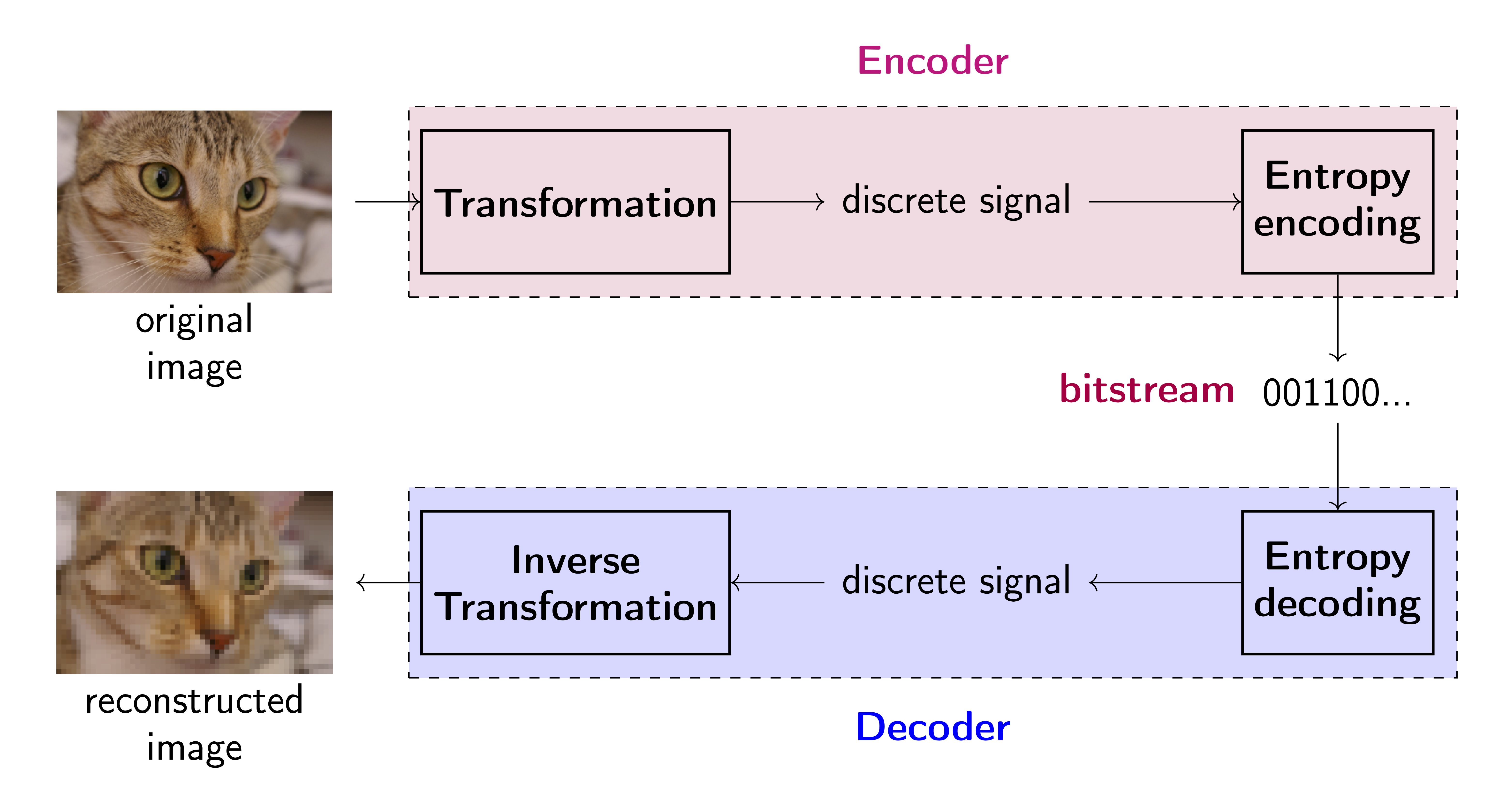
This notes is about the compression algorithms including typical compression models and neural comression models. The length of a message representing some data is proportional to the entropy of this data. In compression tasks, our goal is to design a bitstream such that a uniquely decodable code whose expected length is as close as possible to the entropy of the original data.

Background

The goal of data compression is to represent a given sequence $a_1,\cdots, a_n$ produced by a source as a sequence of bits of minimal possible length. The main reason for the possibility of data compression is the experimental (empirical) law: real-world sources produce very restricted sets of sequences. The compression problem can be formulated as a search problem: given a source, find the shortest possible code for the source2.

source: https://jmtomczak.github.io/blog/8/compression_scheme.png

Problem Formulation

Given one random variable $X\sim P_X$, our goal is to represent it in term of bits efficiently.

Lossless: variable-length code, uniquely decodable codes, prefix codes, Huffman codes

Note: Lossless compression is only possible for discrete R.V.;

$$ P(X\neq \hat{X})=0 $$

Almost lossless: fixed-length code, arithmetic coding

$$ P(X\neq \hat{X})\leq \epsilon $$

Lossy: quantization, vector quantization, predictive coding

$$ X \rightarrow W \rightarrow \hat{X} \text{ s.t.} E[(X-\hat{X})^2]\leq \text{distortion}. $$

Notation:

Codeword: a sequence of bits that represents a symbol $f(x)\in\{0,1\}^*:=\{\emptyset,0,1,00,01,\cdots\}$
Codebook: a set of codewords $\{f(x):x\in\mathcal{X}\}\subset \{0,1\}^*$
WLOG, we can relabel $X$ such that $X = \mathbb{N} = \{1,2,…\}$ and order the pmf decreasingly: $P_{X}(i) \geq P_{X}(i + 1)$
Length function: $l:\{0,1\}^*\rightarrow \mathbb{N}$; e.g., $l(01001)=5$.
Stochastic dominance: $Y$ stochastically dominates (or, is stochastically larger than) $X$, denoted by $X\stackrel{\text{st.}}{\leq} Y$, if $\operatorname{Pr}(Y\leq t)\leq \operatorname{Pr}(X\leq t)$ for all $t\in \mathbb{R}$.

Standard Compression Techniques

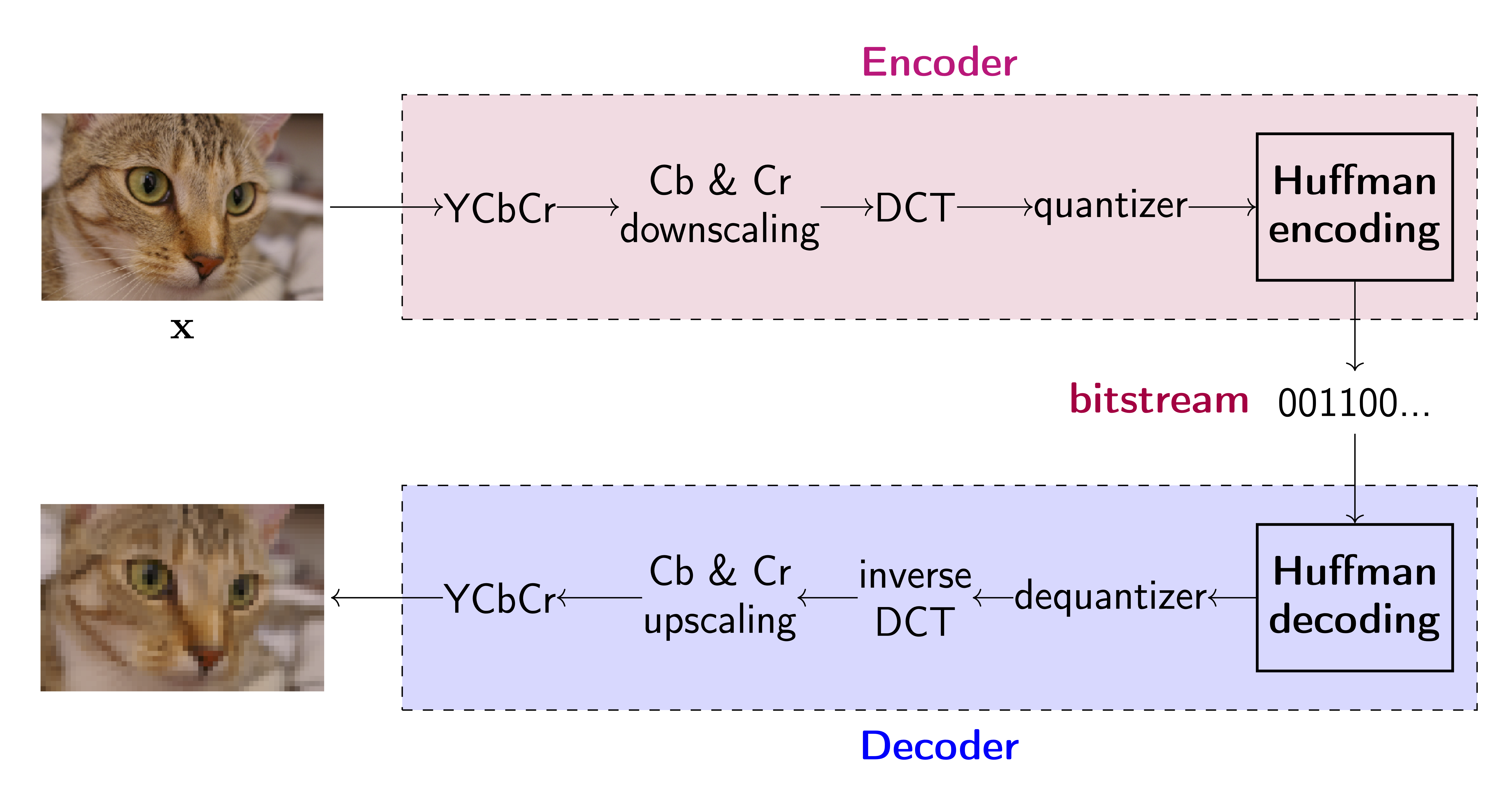
Many popular traditional compression techniques including JPEG, PNG, etc. mainly use hand-designed math tools in each step to encode and decode the signals. Jakub M. Tomczak’s blog 1 introduces a little bit about the working details of JPEG (as shown below), which consists of few linearly transformation and discrete cosine transform (DCT) steps. Also please refer to Balle’s paper for more details.

JPEG source: https://jmtomczak.github.io/blog/8/jpeg_scheme.png

Quantization and Entropy coding

Why do we need to quantize the signal?

Quantization is a process of mapping a continuous signal to a discrete signal. The main reason for quantization is to reduce the number of bits needed to represent the signal. The quantization process is usually followed by entropy coding, which is a process of mapping a discrete signal to a bitstream. The main reason for entropy coding is to reduce the redundancy of the bitstream.

The data is saved in bits in computer, we usually use bit per pixel (BBP) to represent how many bits are needed to represent each pixel. A floating number is represented by 32 bits, which is 4 bytes. If we use an integer (which takes 8 bits) to represent each pixel, we can save 4 times of space. Thus we need to quantize the floating number to a discrete signal first, and then use entropy coding to map the discrete signal to a bitstream.

For compression tasks, we often have to make a trade-off between compression rate (e.g., BPP) and the distortion error (e.g., SSIM, PSNR, etc.), which is well-known as the rate-distortion problem4. $$ \inf_{P_{Y|X}} I(Y;X) \quad \text{s.t. } D\leq D^*$$

How to achieve smaller BBP?

Lets condier the following example5: given an image with size 768*512, if we use deep neural network to generate compressed feature with size 96*64*192 data units. If each data unit needs to consume an average of 1 bits, 96*64*192 bits are needed to encode the entire image. Therefore, the bbp is (96*64*192*1)/(768*512)=3, i.e., 3 bit/pixel. Among which, 96*64*192 is determined by the designed feature encoder, and 1 is realated to the rate of entropy coding. If we make the pmf of the compressed feature data unit be concentrated as much as possible, and the value range as small as possible, so that we can further reduce the value of 1 through entropy coding, and the image compression rate will be further improved.

Neural Compression

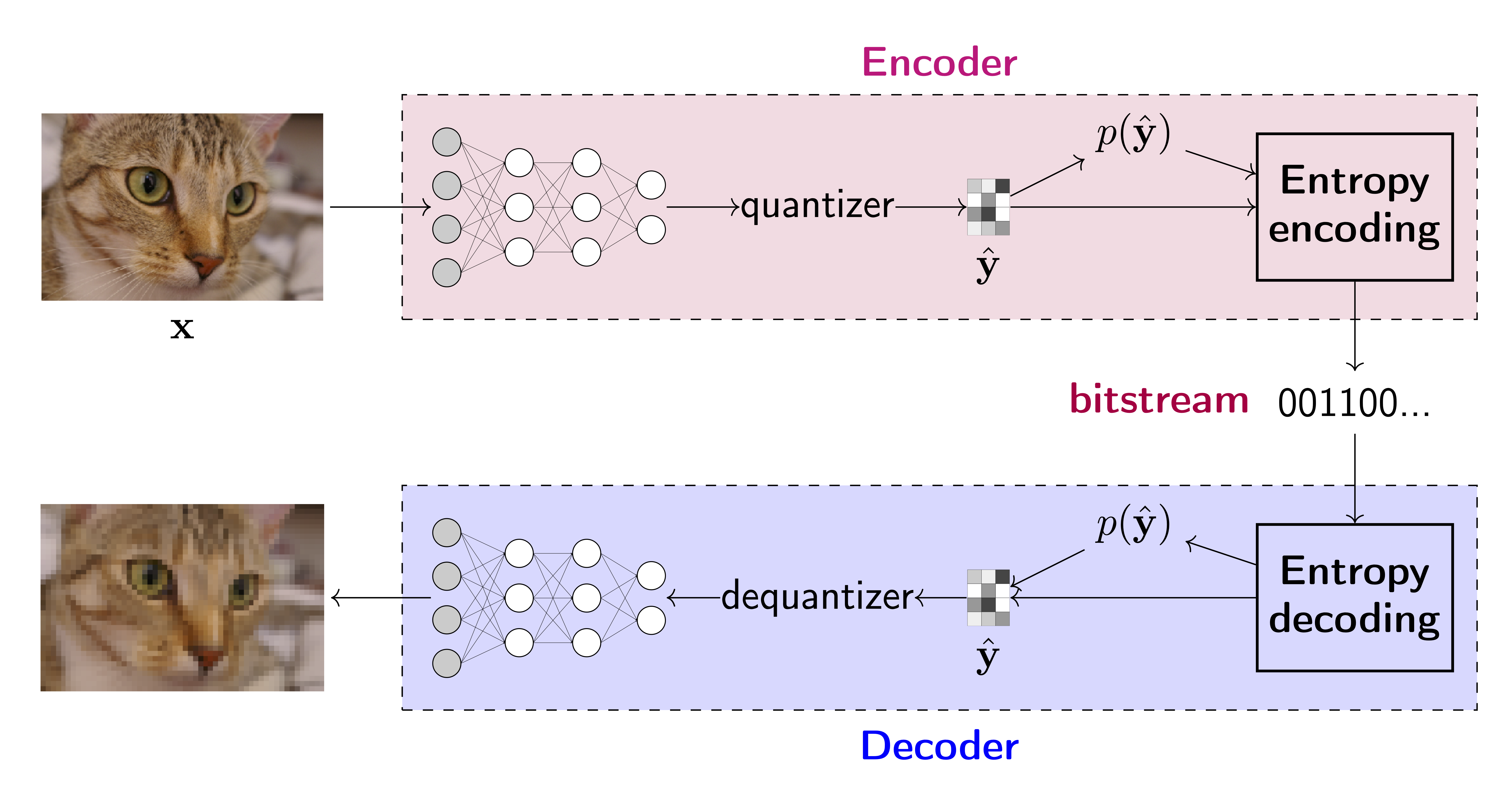
With the powerful capability of neural networks, we can also design end-to-end neural compression models which may achieve better compression rate than DTC or Wavelet Transform (WT). The following figure shows the general structure of a neural compression model.

neu_compression source: https://jmtomczak.github.io/blog/8/neural_compression_scheme.png